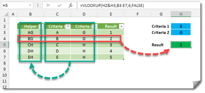
How do you use VLOOKUP with multiple lookup criteria? In its basic form, VLOOKUP can only look up data based on one criteria. To get around this, you could add in another helper column that concatenates the different criteria together and then looks up data based on that.
You formula might look something like this. Using array formula plus the CHOOSE function we can avoid this workaround and keep our data tables less cluttered.
In this example we use =VLOOKUP(G2&G3,CHOOSE({1,2},B3:B7&C3:C7,D3:D7),2,FALSE) and instead of pressing enter, hold down Ctrl and Shift then press Enter. This will enter the formula as an array formula and you will see curly brackets {} around it in the formula editor bar.
Remember to press Ctrl + Shift then Enter to create an array formula.